As rabbit holes usually are, you never expect falling into them. I watched a YouTube video, took a Graph Algorithms class, and then found myself working on a long-term graph visualization engine.

Why visualize graphs?

Many ideas in graph theory hurt to think about and explain, but are highly intuitive when you see a picture. K-core, community detection, and chordal graphs are all terms that would not make sense to someone who doesn't know the graph theory behind them. However, when looking at an image of the graph, humans are very good at spotting patterns, even if they don't know the jargon to describe what they're noticing. To add to this, there is something oddly satisfying about creating a picture anyone can understand from such an abstract data structure.

There is much to be gained from the ability to see such abstract structures, other than seeing what the Internet looks like, or watching spring simulations converge.

Graph visualization is often used in fraud-detection in financial applications, visualizing how money flows between users. Or connecting a group of users who share an absurd amount of identifiers (cookies, fingerprints, etc.). Though the graph layouts are usually only as useful as the quality of the input graph data, they can still give a lot of information with no data analysis work.

Different classes and sizes of graphs call for differently shaped drawings. And different algorithms can produce highly different drawings for the same input graph. Each algorithm usually defines a set of aesthetics it achieves and guarantees. This means the embedding engine should provide many options for layout algorithms, such that the user can correctly decide on which one fits their graph data best.

A graph in and of itself is a pure mathematical structure with no idea of geometry. Having to go from this structure to a drawing can be a daunting experience through the abstract. Such layout algorithms are deterministic and work on combinatorial ideas in graph theory. For this post, I will avoid exploring these types of algorithms as they are far too in-depth, and would require going over too many prerequisites. Fear not, however, as there are many other methods I'll explore.

Force-Directed Framework

Instead of using pure graph theoretical methods, it turns out that we can elegantly model the graph layout problem as an n-body physics simulation. This can take out all the involved algorithms and replace them, mostly, with two primitives that define the final layout, repulsive forces, applied globally between all vertices, and attractive forces, applied only between vertices with an edge between them.

The two functions which define the force magnitudes, and how they are used and scaled, in turn define the whole layout. And while anything can be used for them, through the years of research a few became standards. Most of which are usually modeled after real-world force functions that show up in similar n-body problems.

While the possible functions are endless, ranging from those based on Coulomb's law to spring physics, a general model made by Noack proposed a way to easily classify them. In general, force models can be defined by a tuple (a, r), where a and r are the exponents of the distance variable in the attractive and repulsive force functions.

Depending on how the two exponents relate to each other in terms of growth, the result can be very different output layouts. You can get separated clumps of vertices, or add constants to the force equations to control the edge length.

For example, the Fruchterman-Reingold force equation has the tuple (2, -1), and defines an ideal edge length k.

$$ f_a(d) = \frac{d^2}{k}, \qquad f_r(d) = \frac{k^2}{d} $$

Solving for equilibrium, we see that this is achieved once the distance is equal to the ideal edge length. And in cases where the distance is smaller, repulsion starts increasing quickly, while attraction decreases. And the opposite happens when the vertices are too far apart.

If we begin by placing all vertices in random positions and running the forces until equilibrium, we'll get stable layouts that look like this:

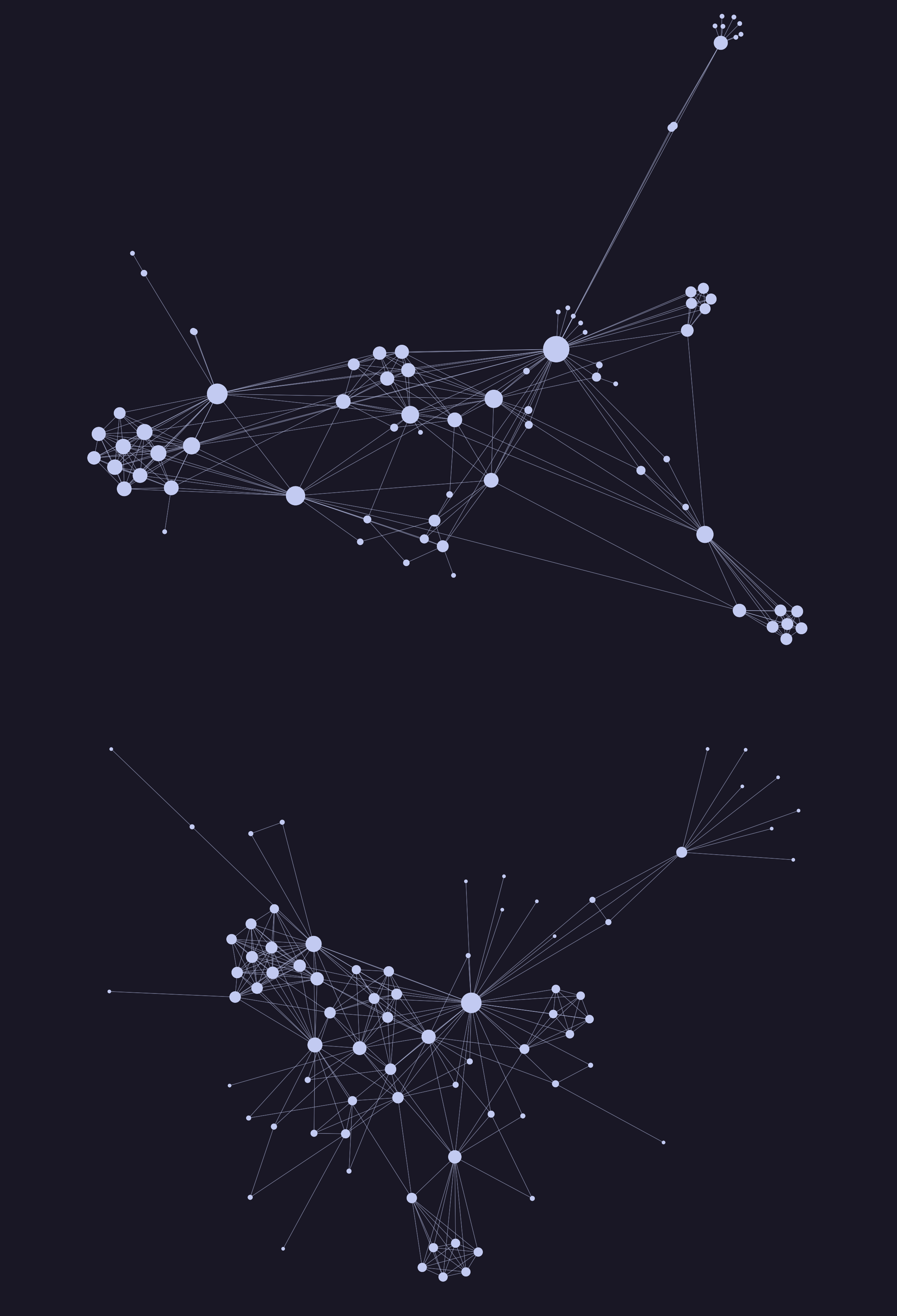
We can see how the top layout, drawn using Noack's LinLog force model, leads to visual clustering and separation between clusters. The nodes that connect these clusters are called hubs, and they are what this force model wants to highlight. While in the bottom Fruchterman-Reingold layout, we have more uniform edge lengths, which come from the ideal edge length constant in the function.

While the differences between the outputs are interesting, one shared drawback is present among all force models. That is the O(|V|^2) time complexity that comes with pairwise force calculations. So, I'll show you some significant optimization algorithms I've run into which help mitigate this time complexity.

Barnes-Hut

The basic force-directed algorithm would calculate repulsion forces between all pairs of vertices. While this is needed to avoid collapsing vertices, we may not need to calculate the forces for all pairs. If we have a vertex that is far away from a cluster of vertices, we can opt to treat that entire cluster as one body instead. This would save us a lot of work, while also keeping some approximate accuracy.

Barnes-Hut does this optimization as an addition to force-directed models. It takes the time complexity down to O(|V|log(|V|)), while keeping the loop structure the same.

It achieves this by maintaining a spatial index data structure of the plane, commonly a quadtree. With this, we can approximate these distant vertices as one massive body when calculating repulsive forces. We should also scale that force vector by the number of vertices in the quadtree node.

We construct the quadtree such that leaf nodes only include 1 vertex. For a given vertex V, we calculate its repulsive forces like so, with variables theta a constant, node initially set to the quadtree root, and vPos V's position:

1. If node is a leaf, we calculate the repulsive force normally, as it only contains 1 vertex.
2. We calculate a ratio = node.width / dist, where dist is the distance between the center of mass of the node and vPos. And node.width is simply how wide the quadtree node is.
3. If the ratio < theta, we treat the quadtree node as one vertex and calculate repulsive forces against its center of mass.
4. Otherwise, we repeat recursively on each child node.

void ForceAtlas::AccumulateBHRepulsion(const QuadTree::Node *node,
                                       size_t selfIdx, const double *vPos,
                                       double *acc) const {
  // forces are accumulated in acc

  if (!node || node->Mass() == 0.0) // empty
    return;

  if (node->IsLeaf()) {
    // only one vertex in the quadtree node, by construction
      size_t idx = node->PointAt(0); 
      if (idx == selfIdx)
        return;
      const double *uPos = positions_.data() + idx * 2;
      model_->Repulsive(vPos, uPos, mass_[selfIdx], mass_[idx], acc);
    return;
  }

  double comX, comY;
  node->CenterOfMass(&comX, &comY);
  double dx = comX - vPos[0];
  double dy = comY - vPos[1];
  double dist = std::sqrt(dx * dx + dy * dy);
  double ratio = (2.0 * node->HalfSize()) / dist;

  if (ratio < theta_) {
    double com[2] = {comX, comY};
    model_->Repulsive(vPos, com, mass_[selfIdx], node->Mass(), acc);
    return;
  }

  for (size_t q = 0; q < QuadTree::kQuadrantCount; q++)
    AccumulateBHRepulsion(node->Child(static_cast<QuadTree::Quadrant>(q)),
                           selfIdx, vPos, acc);
}

This clever modification to how the repulsive forces are calculated takes algorithms from being unrunnable on large graphs to running smoothly. A 10,000-vertex graph takes 23ms to run a single force iteration without Barnes-Hut, and 4ms with!

Additionally, the fact that Barnes-Hut is agnostic of the force model being used makes it essentially a free on/off switch for optimization!

Graph Drawing with Intelligent Placement

While Barnes-Hut can provide enormous speedups for the most general graphs, some graphs are still too large for it. We need to approach such graphs in a creative way, improving further on the usual force-directed methods. Algorithms optimized for this are different from Barnes-Hut, as they are not a simple plug-and-play optimization. Instead, they usually define their own pipeline to produce a layout.

One such example is Graph Drawing with Intelligent Placement (GRIP). It falls under a category of algorithms called multilevel layout algorithms. These work by subdividing the input graph into a sequence of subgraph levels, such that the deeper levels would be easier to work with, and allow us to cheaply propagate information to build the full layout.

GRIP works by dissecting the input graph vertices (we'll call this set V) into multiple subsets V = V0 > V1 > ... > Vn. It defines this dissection in an intricate way called the Maximal Independent Set (MIS) filtration of the graph's vertices. In such a filtration, the final layers will have a small number of vertices, which we'll place using force-directed methods. And then we use the layout of each layer Vi as a base for the layout of Vi-1.

A filtration is an MIS filtration if it satisfies the following properties. Each layer is a subset of the layer before it. For any two vertices in a layer Vi, the graph distance between them must be larger than 2^(i-1). Equivalently, we write:

$$ \forall i<n, \quad V_i \subset V_{i-1} $$ $$ \wedge \quad \forall u, v \in V_i, \quad \text{dist}(u, v) > 2^{i-1} $$

To construct it, we use repeated Breadth First Searches: pick an unvisited vertex, keep it, and mark everything within the radius as unpickable. This ensures the distance constraint at each layer. And we keep repeating this until all vertices are marked.

bool GRIP::IterMISFiltration(size_t i, BitSet &prevSubset) {
  // the index of the layer we are building is i
  // the previous layer we've built is prevSubset

  size_t nvertices = Structure().VertexCapacity();
  BitSet newSubset(nvertices);
  BitSet marked(nvertices);

  size_t radius = size_t{1} << (i - 1);

  // iterate over the vertices present in prevSubset.
  for (size_t curr : prevSubset) {
    if (marked.Test(curr)) {
      continue;
    }

    // mark as part of the new subset, and as unchoosable.
    newSubset.Set(curr);
    marked.Set(curr);

    // VerticesWithinRadius performs a BFS from curr with maxDepth 
    // radius, and sets the reached vertices in the marked BitSet.
    VerticesWithinRadius(curr, radius, marked);
  }

  // newSubset will now store the next MIS layer's vertices 

  ...
}

Notice, also, while the final layers of the filtration run a BFS with a large maximum depth, the number of vertices in those layers will be very small, keeping the amount of work done manageable. Similarly, the first few layers have many vertices, but only a very shallow BFS.

With our MIS filtration created, we can place the last layer in a simple shape, such as a triangle for 2D or a tetrahedron for 3D. We can ensure that the final layer has the correct number of vertices for the simplex by migrating vertices between the final two layers.

From there, we iterate over the layers in reverse order and, for each layer Vi, we take the following two-phase process:

1. This phase is the namesake of the algorithm, intelligent placement. For each vertex V in Vi but not Vi+1, we place V at the average position of its K-nearest neighbors in Vi+1.
2. The second phase is local refinement. For ALL the vertices in Vi, we calculate attractive and repulsive forces with its K-nearest neighbors. We run the refinement for multiple rounds.

These K-nearest neighbors are calculated in terms of graph distance, and allow the force and position calculations to be much cheaper than if they were global.

That's it! After running these two phases on all layers, the final layout is produced. The two simple phases, which all perform local updates with no knowledge of global state, give us the following guarantees:

1. The initial position of each vertex will be near its position in the final layout.
2. All global structures and symmetries of the graph will appear in the final layout, even though all updates were local!

All of this is done in O(|V|) time and space complexity! And it produces some mind-blowing outputs:

Trees

Visualizing trees is an extremely common place for graph visualization to show up. As opposed to the layout of general graphs, tree layouts have been mathematically solved and optimized to use the least amount of space possible, all while looking neat. While you can use normal force-directed methods, there are mathematical visualizers which are deterministic and have concrete guarantees. In fact, you have probably used such tree visualizers regularly.

The tree command can visualize a subtree of your file system and draw it to the terminal. While no fancy rendering or physics is being done, it gives useful and readable detail about the hierarchical structure of your directory.

% tree -L 2
.
├── CLAUDE.md
├── CMakeLists.txt
├── compile_commands.json
├── include
│   ├── BitSet.hpp
│   ├── BreadthFirst.hpp
│   ├── ConnectedComponents.hpp
│   ├── DepthFirst.hpp
│   ├── EmbeddedGraph.hpp
    ...
├── README.md
├── src
│   ├── BreadthFirst.cpp
│   ├── ConnectedComponents.cpp
│   ├── DepthFirst.cpp
│   ├── EmbeddedGraph.cpp
│   ├── ForceAtlas.cpp
│   ├── Graph.cpp
    ...
└── third-party
    ├── boyerMyrvold
    ├── msf_gif.h
    └── unity

Force-Directed Tree Layouts

Before we dive into how such a layout is produced, let's experiment and see how our force-directed methods fare against this class of graphs.

The tree command, and other tree layout algorithms, give extremely normalized drawings regardless of the tree shape. This is in part due to the fact that they rely on deterministic mathematical processes to find vertex offsets. However, using our force-directed methods produces interesting layouts.

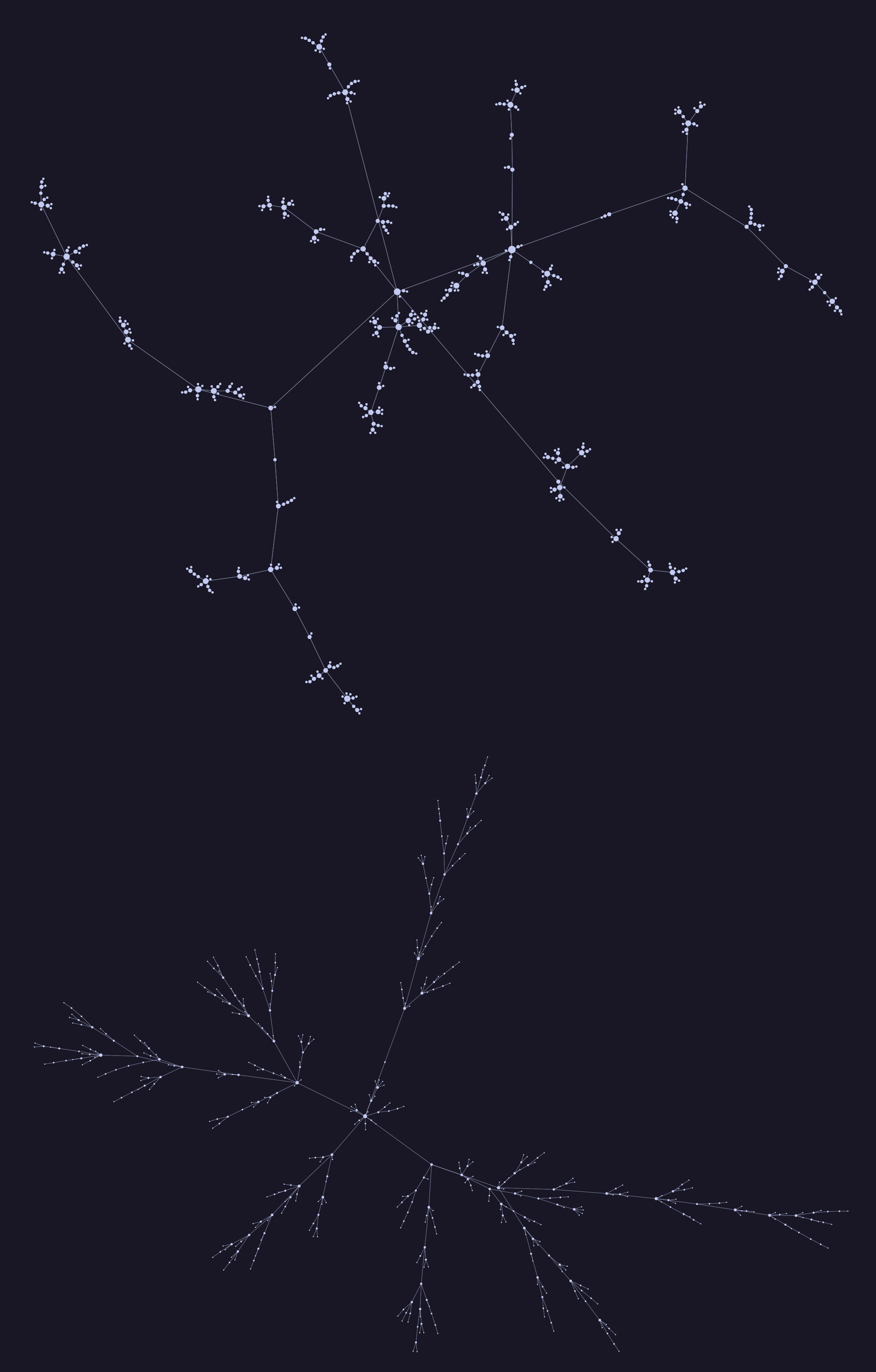
We can see LinLog's hub separation, covered in the beginning of the post, playing a big role here. Vertices which are significant branching points are clearly isolated and highlighted in the drawing. And, in contrast, leaves are tucked close to their parents.

While in the Fruchterman-Reingold layout, we see a much more natural-looking tree structure. This is, in part, due to the similarity in edge lengths. This spiky look is a common sight for Fruchterman-Reingold layouts, and we get control over its extent via the edge length parameter k.

While both layouts are quite pretty, they do throw away an important detail. The hierarchical structure of trees is completely disregarded in these algorithms' specifications. And thus, in some cases, it makes it hard to discern, for example, where the root is or which direction goes up the tree.

Reingold-Tilford Algorithm

Algorithms like the one behind tree solve the issue we've seen nicely by encoding the parent-child relation in an axis of its own. And, when visualizing user-facing layouts for small trees, for example when showing Kubernetes deployments in a tool like ArgoCD, this information is often extremely useful. Additionally, they do this in a way that is deterministic, gives similar shapes across trees, and is instant, i.e., no "wait for the forces to settle" phase.

While the tree command is nice, we can extend its recursive approach to get more regular drawings. We'll look at an extended version of the Reingold-Tilford (RT) algorithm (the original RT algorithm only supports binary trees) which does just that. This algorithm gives us strong guarantees for the shape of the output:

1. Vertices at the same depth level of the tree should lie along a straight line, and the straight lines defining the levels should be parallel.
2. The children of a vertex should appear in their adjacency-list order, left to right.
3. A parent should be centered over its children.
4. A tree and its mirror image should produce drawings that are reflections of one another; moreover, a subtree should be drawn the same way regardless of where it occurs in the tree.

The last two of which are not achieved by tree. Reingold and Tilford propose an O(|V|) algorithm to achieve all of them, which has become a standard.

The y-axis is trivial, as it is simply the depth of each node multiplied by some scaling factor. To find x-axis positions, the algorithm calculates the relative x-offsets in each subtree independently. This independence is what ensures aesthetic (4) is achieved, since no global state is required to find what any one subtree will look like.

To get an idea of what these aesthetic guarantees give us, let's visualize another 500-vertex tree with RT:

It produces an extremely normal and optimally packed layout. However, since one axis is scaling with depth and the other is scaling with branching, our layout is extremely wide. Because vertex count naturally scales exponentially with depth, this is an unavoidable limitation of such tree layout algorithms.

The algorithm follows a divide-and-conquer approach through a post-order traversal of the tree (children left-to-right then parent), and places each node's subtree independently before merging them together.

void ReingoldTilford::CalculateOffsets(size_t root, size_t level) {
  size_t degree = graph_.Degree(root);

  // Divide
  for (size_t i = 0; i < degree; i++)
    CalculateOffsets(graph_.Neighbor(root, i), level + 1);

  // Initialization. Includes base case (leaf node)
  InitializeRTSubtreeRoot(root, level);

  // Conquer
  for (size_t i = 0; i < degree; i++)
    CombineSubtreeLeft(root, i);
}

As is usual, the base case (a node with no children) is trivial. It is simply placed with no child offsets to calculate. After that, when non-leaves are reached in the traversal, they are combined based on a contour-walk.

CombineSubtreeLeft(root, child) takes a subtree root and its parent. It calculates the minimum x-coordinate distance between the parent's children, up to the subtree root, such that the subtree does not overlap with any of its left siblings. It repeats this in a loop until all children are merged in, and stores x-coordinate offsets for each of the parent's children. This is the main conquer step, and I think the details are best explained through a real-world analogy and an accompanying animation :).

First, with your child subtrees each drawn on a piece of paper (which happens in the previous recursive calls that returned), cut along the left and right boundaries of each subtree. Each silhouette of a subtree is made up of the left and right contours, where the contours of a subtree are defined as the leftmost/rightmost vertex at each of its depth layers. We'll place the first child directly under the parent, and begin merging from the second child.

When merging a subtree with its left siblings, begin by overlapping its root with the sibling directly to its left. Then, you walk the right contour of the left subtree and left contour of the right subtree in lockstep, and calculate the x-coordinate difference between the contour vertices at each step. If that difference is less than a constant minimum distance, you add the difference to the separation. You repeat this process until you reach the bottom of either contour.

The tricky part is that most trees will have unequal depths, so the two contours being compared will usually have one side reach a leaf before the other is done walking its contour. The fix is threading. When a contour walk hits a leaf on the shallow side while the other side still has levels left, it creates a thread, a temporary fake edge, from that leaf down to the next vertex on the deeper contour.

These threads effectively merge the subtree with its siblings, so that later walks that pass through the leaf will now follow the thread. This will make the shallow subtree's contour behave as if it extended all the way down. These threads are purely a bookkeeping tool, and are usually stored via gross pointer repurposing.

Once all children are merged this way, the parent is simply placed centered on the calculated relative offsets of its children.

These offsets are still relative to each node's own parent though, so a second pass, this time top-down from the root, walks the tree once more accumulating each node's offset with its parent's to produce final absolute coordinates.

Is that all?

Not even close. Though what I've covered here forms the base of many significant algorithms, it is not yet enough for any graph.

There are graphs that live on a scale which none of the algorithms I've covered visualize well. The Wikipedia graph, for example, can be run through GRIP, but results in what's called a "hairball," with many edges covering the screen and no value to be gained. These graphs, which lack global structure and are dense in edges, are the kryptonite of GRIP.

Also, more aesthetics can be achieved. In force-directed graphs, you are not restricted to normal N-dimensional spaces. We are able to visualize graphs on donuts! These are the improvements I'm currently looking to add to my library, but more exist.

The point here is that graph visualization is an entire field, where creatively applying concepts from neighboring maths can lead to jaw-dropping images that tell stories.

The code snippets throughout this article are taken from my library gviz, which is actively being worked on to implement these niche visualizers. When I began working on it, I certainly did not expect to stay as long as I did. And I did not expect to become a person always looking out for graphs to visualize.